SQL Server 2012 : Query Plans (part 3) - Reading Query Plans

Reading Query Plans

Once you have downloaded and installed the sample database, to make the examples more interesting you need to remove some of the indexes that the authors of AdventureWorks added for you. To do this, you can use either your favorite T-SQL scripting tool or the SSMS scripting features, or run the AW2012_person_drop_indexes.sql sample script. This script drops all the indexes on the person.person table except for the primary key constraint.

After you have done this, you can follow along with the examples, and you should see the same results.

You will begin by looking at some trivial query plans, starting with a view of the graphical plans but quickly switching to using the text plan features, as these are easier to compare against one another, especially when you start looking at larger plans from more complex queries.

Here is the first trivial query to examine:

select firstname, COUNT (*)
from Person.Person
group by firstname
order by COUNT (*) desc

After running this in SSMS after enabling the Include Actual Execution Plan option, which is shown in Figure 7, three tabs are displayed. The first is Results, but the one you are interested in now is the third tab, which shows the graphical execution plan for this query.

FIGURE 7

You should see something like the image shown in Figure 8.

FIGURE 8

Starting at the bottom right, you can see that the first operator is the clustered index scan operator. While the query doesn’t need, or get any benefit from, a clustered index, because the table has a clustered index and is not a heap, this is the option that SQL Server chooses to read through all the rows in the table. If you had removed the clustered index, so that this table was a heap, then this operator would be replaced by a table scan operator. The action performed by both operators in this case is identical, which is to read every row from the table and deliver them to the next operator.

The next operator is the hash match. In this case, SQL Server is using this to sort the rows into buckets by first name. After the hash match is the compute scalar, whereby SQL Server counts the number of rows in each hash bucket, which gives you the count (*) value in the results. This is followed by the sort operator, which is there to provide the ordered output needed from the T-SQL.

You can find additional information on each operation by hovering over the operator. Figure 9 shows the additional information available on the non-clustered index scan operator.

FIGURE 9

While this query seems pretty trivial, and you may have assumed it would generate a trivial plan because of the grouping and ordering, this is not a trivial plan. You can tell this by monitoring the results of the following query before and after running it:

select *
from sys.dm_exec_query_optimizer_info
where counter in (
'optimizations'
, 'trivial plan'
, 'search 0'
, 'search 1'
, 'search 2'
)
order by [counter]

Once the query has been optimized and cached, subsequent runs will not generate any updates to the Query Optimizer stats unless you flush the procedure cache using dbcc freeproccache.

On the machine I am using, the following results were returned from this query against the Query Optimizer information before I ran the sample query:

COUNTER         OCCURRENCE  VALUE
optimizations   10059       1
search 0        1017        1
search 1        3385        1
search 2        1           1
trivial plan    5656        1

Here are the results after I ran the sample query:

COUNTER         OCCURRENCE  VALUE
optimizations   10061       1
search 0        1017        1
search 1        3387        1
search 2        1           1
trivial plan    5656        1

From this you can see that the trivial plan count didn’t increment, but the search 1 count did increment, indicating that this query needed to move onto phase 1 of the optimization process before an acceptable plan was found.

If you want to play around with this query to see what a truly trivial plan would be, try running the following:

select lastname 
from person.person

The following T-SQL demonstrates what the same plan looks like in text mode:

set statistics profile on
go
 
select firstname, COUNT (*)
from Person.Person
group by firstname
order by 2 desc
go
 
set statistics profile off
go

When you run this batch, rather than see a third tab displayed in SSMS, you will see that there are now two result sets in the query’s Results tab. The first is the output from running the query, and the second is the text output for this plan, which looks something like what is shown in Figure 10.

FIGURE 10

---

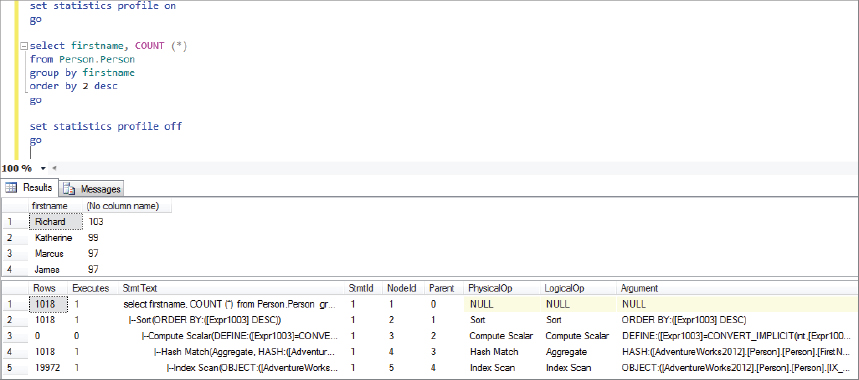
The following example shows some of the content of the StmtText column, which illustrates what the query plan looks like, just as in the graphical plan but this time in a textual format:

  |--Sort(ORDER BY:([Expr1003] DESC))
       |--Compute Scalar(DEFINE:([Expr1003 ...
            |--Hash Match(Aggregate, ...
                 |--Index Scan(OBJECT:( ...

As mentioned before, this is read from the bottom up. You can see that the first operator is the clustered index scan, which is the same operator shown in Figure 1. From there (working up), the next operator is the hash match, followed by the compute scalar operator, and then the sort operator.

While the query you examined may seem pretty simple, you have noticed that even for this query, the Query Optimizer has quite a bit of work to do. As a follow-up exercise, try adding one index at a time back into the Person table, and examine the plan you get each time a new index is added. One hint as to what you will see is to add the index IX_Person_Lastname_firstname_middlename first.

From there you can start to explore with simple table joins, and look into when SQL Server chooses each of the three join operators it offers: nested loop, merge, and hash joins.