SQL Server 2008 R2 : Query Analysis - Query Statistics

In addition to the IO and TIME statistics, SQL Server also provides the SET STATISTICS PROFILE and SET STATISTICS XML options. These options are provided to display execution plan information while still allowing the query to run.

STATISTICS IO

You can set the STATISTICS IO option for individual user sessions, and you can turn it on in an SSMS query window by typing the following:

SET STATISTICS IO ON
GO

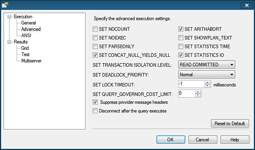
You can also set this option for the query session in SSMS by choosing the Options item in the Query menu. In the Query Options dialog, click the Advanced item and check the SET STATISTICS IO check box, as shown in Figure 1.

Figure 1. Enabling the STATISTICS IO option in SSMS.

The STATISTICS IO option displays the scan count (that is, the number of iterations), the logical reads (from cached data), the physical reads (from physical storage), and the read-ahead reads.

Listing 1. An Example of STATISTICS IO Output

set statistics io on
go
select st.stor_name, ord_date, qty
from stores st join sales_noclust s on st.stor_id = s.stor_id
where st.stor_id between 'B100' and 'B199'
go

-- output deleted

(1077 row(s) affected)
Table 'sales_noclust'. Scan count 100, logical reads 1383, physical reads 5,
 read-ahead reads 8, lob logical reads 0, lob physical reads 0,
 lob read-ahead reads 0.
Table 'stores'. Scan count 1, logical reads 3, physical reads 0,
 read-ahead reads 0, lob logical reads 0, lob physical reads 0,
 lob read-ahead reads 0.


					  

Scan Count

The scan count value indicates the number of times the corresponding table was accessed during query execution. The outer table of a nested loop join typically has a scan count of 1. The scan count for the inner tables typically reflects the number of times the inner table is searched, which is usually the same as the number of qualifying rows in the outer table. The number of logical reads for the inner table is equal to the scan count multiplied by the number of pages per lookup for each scan. Note that the scan count for the inner table might sometimes be only 1 for a nested join if SQL Server copies the needed rows from the inner table into a work table in cache memory and reads from the work table for subsequent iterations (for example, if it uses the Table Spool operation). The scan count for hash joins and merge joins is typically 1 for both tables involved in the join, but the logical reads for these types of joins are usually substantially higher.

Logical Reads

The logical reads value indicates the total number of page accesses necessary to process the query. Every page is read from cache memory, even if it first has to be read from disk. Every physical read always has a corresponding logical read, so the number of physical reads will never exceed the number of logical reads. Because the same page might be accessed multiple times, the number of logical reads for a table could exceed the total number of pages in the table.

Physical Reads

The physical reads value indicates the actual number of pages read from disk. The value for physical reads can vary greatly and should decrease, or drop to zero, with subsequent executions of the query because the data will be loaded into the data cache by the first execution. The number of physical reads will also be lowered by pages brought into memory by the read-ahead mechanism.

Read-Ahead Reads

The read-ahead reads value indicates the number of pages read into cache memory using the read-ahead mechanism while the query was processed. Pages read by the read-ahead mechanism will not necessarily be used by the query. When a page read by the read-ahead mechanism is accessed by the query, it counts as a logical read, but not as a physical read.

The read-ahead mechanism can be thought of as an optimistic form of physical I/O, reading the pages into cache memory that it expects the query will need before the query needs them. When you are scanning a table or index, the table’s index allocation map pages (IAMs) are looked at to determine which extents belong to the object. An extent consists of eight data pages. The eight pages in the extent are read with a single read, and the extents are read in the order that they are stored on disk. If the table is spread across multiple files, the read-ahead mechanism attempts parallel reads from up to eight files at a time instead of sequentially reading from the files.

LOB Reads

If the query retrieves text, ntext, image, or large value type (varchar(max), nvarchar(max), varbinary(max)) data, the lob logical reads, lob physical reads, and lob read-ahead reads values provide the logical, physical, and read-ahead read statistics for the large object (LOB) I/Os.

Analyzing STATISTICS IO Output

The output shown in Listing 36.4 indicates that the sales_noclust table was scanned 100 times, with 5 physical reads (that is, 5 physical I/Os were performed). The stores table was scanned once, with all reads coming from cache (physical reads = 0).

You can use the STATISTICS IO option to evaluate the effectiveness of the size of the data cache and to evaluate, over time, how long a table will stay in cache. The lack of physical reads is a good sign, indicating that memory is sufficient to keep the data in cache. If you keep seeing many physical reads when you are analyzing and testing your queries, you might want to consider adding more memory to the server to improve the cache hit ratio. You can estimate the cache hit ratio for a query by using the following formula:

Cache hit ratio = (Logical reads – Physical reads) / Logical reads

The number of physical reads appears lower than it actually is if pages are preloaded by read-ahead activity. Because read-ahead reads lower the physical read count, they give the indication of a good cache hit ratio, when in actuality, the data is still being physically read from disk. The system could still benefit from more memory so that the data remains in cache and the number of read-ahead reads is reduced. STATISTICS IO is generally more useful for evaluating individual query performance than for evaluating overall cache hit ratio. The pages that reside and remain in memory for subsequent executions are determined by the data pages being accessed by other queries executing at the same time and the number of data pages being accessed by the other queries. If no other activity is occurring, you are likely to see no physical reads for subsequent executions of the query if the amount of data being accessed fits in the available cache memory. Likewise, if the same data is being accessed by multiple queries, the data tends to stay in cache, and the number of physical reads for subsequent executions tends to be low. However, if other queries executing at the same time are accessing large volumes of data from different tables or ranges of values, the data needed for the query you are testing might end up being flushed from cache, and the physical I/Os will increase. Depending on the other ongoing SQL Server activity, the physical reads you see displayed by STATISTICS IO can be inconsistent.

When you are evaluating individual query performance, examining the logical reads value is usually more helpful because the information is consistent across all executions, regardless of other SQL Server activity. Generally speaking, the queries with the fewest logical reads are the fastest queries. 

STATISTICS TIME

You can set the STATISTICS TIME option for individual user sessions. In an SSMS query window, you type the following:

SET STATISTICS TIME ON

You can also set this option for the query session in SSMS by choosing the Options item in the Query menu. In the Query Options dialog, you click the Advanced item and check the SET STATISTICS TIME check box.

The STATISTICS TIME option displays the total CPU and elapsed time that it takes to actually execute a query. 

Listing 2. An Example of STATISTICS TIME Output

set statistics io on
set statistics time on
go

select st.stor_name, ord_date, qty
from stores st join sales_noclust s on st.stor_id = s.stor_id
where st.stor_id between 'B100' and 'B199'
go


SQL Server parse and compile time:
   CPU time = 0 ms, elapsed time = 0 ms.

--output deleted

(1077 row(s) affected)
Table 'sales_noclust'. Scan count 100, logical reads 1383, physical reads 0,
 read-ahead reads 0, lob logical reads 0, lob physical reads 0, lob read-ahead
 reads 0.
Table 'stores'. Scan count 1, logical reads 3, physical reads 0, read-ahead
 reads 0, lob logical reads 0, lob physical reads 0, lob read-ahead reads 0.

 SQL Server Execution Times:
   CPU time = 0 ms,  elapsed time = 187 ms.


					  

Here, you can see that the total execution time, denoted by the elapsed time, was relatively low and not significantly higher than the CPU time. This is due to the lack of any physical reads and the fact that all activity is performed in memory.

If elapsed time is much higher than CPU time, the query had to wait for something, either I/O or locks. If you want to see the effect of physical versus logical I/Os on the performance of a query, you need to flush the pages accessed by the query from memory. You can use the DBCC DROPCLEANBUFFERS command to clear all clean buffer pages out of memory. Listing 36.6 shows an example of clearing the pages from cache and rerunning the query with the STATISTICS IO and STATISTICS TIME options enabled.

Listing 3. An Example of Clearing the Clean Pages from Cache to Generate Physical I/Os

USE bigpubs2008
go
CHECKPOINT
go
DBCC DROPCLEANBUFFERS
go

SET STATISTICS IO ON
SET STATISTICS TIME ON
go
select st.stor_name, ord_date, qty
from stores st join sales_noclust s on st.stor_id = s.stor_id
where st.stor_id between 'B100' and 'B199'
go

SQL Server parse and compile time:
   CPU time = 0 ms, elapsed time = 1 ms.

--output deleted

(1077 row(s) affected)
Table 'sales_noclust'. Scan count 100, logical reads 1383, physical reads 6,
 read-ahead reads 0, lob logical reads 0, lob physical reads 0, lob read-ahead
 reads 0.
Table 'stores'. Scan count 1, logical reads 3, physical reads 2, read-ahead
 reads 0, lob logical reads 0, lob physical reads 0, lob read-ahead reads 0.

 SQL Server Execution Times:
   CPU time = 0 ms,  elapsed time = 282 ms.


					  

Notice that this time around, even though the reported CPU time was the same, the elapsed time was 282 milliseconds due to the physical I/Os that had to be performed during this execution.

You can use the STATISTICS TIME and STATISTICS IO options together in this way as a useful tool for benchmarking and comparing performance when modifying queries or indexes.

Using datediff() to Measure Runtime

Although the STATISTICS TIME option works fine for displaying the runtime of a single query, it is not as useful for displaying the total CPU time and elapsed time for a stored procedure. The STATISTICS TIME option generates time statistics for every command executed within the stored procedure. This makes it difficult to read the output and determine the total elapsed time for the entire stored procedure.

Another way to display runtime for a stored procedure is to capture the current system time right before it starts, capture the current system time as it completes, and display the difference between the two, specifying the appropriate-sized datepart parameter to the datediff() function, depending on how long your procedures typically run. For example, if a procedure takes minutes to complete, you probably want to display the difference in seconds or minutes, rather than milliseconds. If the time to complete is in seconds, you likely want to specify a datepart of seconds or milliseconds. Listing 4 displays an example of using this approach.

Listing 4. Using datediff() to Determine Stored Procedure Runtime

set statistics time off
set statistics io off
go
declare @start datetime
select @start = getdate()
exec sp_help
select datediff(ms, @start, getdate()) as 'runtime(ms)'
go

-- output deleted
runtime(ms)
-----------
         3263

STATISTICS PROFILE

The SET STATISTICS PROFILE option is similar to the SET SHOWPLAN_ALL option but allows the query to actually execute. It returns the same execution plan information displayed with the SET SHOWPLAN_ALL statement, with the addition of two columns that display actual execution information. The Rows column displays the actual number of rows returned in the execution step, and the Executions column shows the actual number of executions for the step. The Rows column can be compared to the EstimatedRows column, and the Execution column can be compared to the EstimatedExecution column to determine the accuracy of the execution plan estimates.

You can set the STATISTICS PROFILE option for individual query sessions. In an SSMS query window, you type the following statement:

SET STATISTICS PROFILE ON
GO

STATISTICS XML

Similar to the STATISTICS PROFILE option, the SET STATISTICS XML option allows a query to execute while also returning the execution plan information. The execution plan information returned is similar to the XML document displayed with the SET SHOWPLAN_XML statement.

To set the STATISTICS XML option for individual query sessions in SSMS or another query tool, you type the following statement:

SET STATISTICS XML ON
GO