In SQL Server 2008, tables are stored in one or more partitions. Partitions
are organizational units that allow you to divide data into logical
groups. By default, a table has only a single partition that contains
all the data. The power of partitions comes into play when you define
multiple partitions for a table that is segmented based on a key column.
This column allows the data rows to be horizontally split. For example,
a date/time column can be used to divide each month’s data into a
separate partition. These partitions can also be aligned to different
filegroups for added flexibility, ease of maintenance, and improved
performance.
The important point to remember is that you access tables with multiple partitions (which are called partitioned tables) the same way you access tables with a single partition. Data Manipulation Language (DML) operations such as INSERT and SELECT
statements reference the table the same way, regardless of
partitioning. The difference between these types of tables has to do
with the back-end storage and the organization of the data.
Generally, partitioning is most useful for large tables. Large
is a relative term, but these tables typically contain millions of rows
and take up gigabytes of space. Often, the tables targeted for
partitioning are large tables experiencing performance problems because
of their size. Partitioning has several different applications,
including the following:
Archival—
Table partitions can be moved from a production table to another
archive table that has the same structure. When done properly, this
partition movement is very fast and allows you to keep a limited amount
of recent data in the production table while keeping the bulk of the
older data in the archive table.
Maintenance—
Table partitions that have been assigned to different filegroups can be
backed up and maintained independently of each other. With very large
tables, maintenance activities on the entire table (such as backups) can
take a prohibitively long time. With partitioned tables, these
maintenance activities can be performed at the partition level.
Consider, for example, a table that is partitioned by month: all the new
activity (updates and insertions) occurs in the partition that contains
the current month’s data. In this scenario, the current month’s
partition would be the focus of the maintenance, thus limiting the
amount of data you need to process.
Query performance—
Partitioned tables joined on partitioned columns can experience
improved performance because the Query Optimizer can join to the table
based on the partitioned column. The caveat is that joins across
partitioned tables not joining on the partitioned column may actually
experience some performance degradation. Queries can also be
parallelized along the partitions.
Now that we have discussed
some of the reasons to use partitioned tables, let’s look at how to set
up partitions. There are three basic steps:
1. | Create a partition function that maps the rows in the table to partitions based on the value of a specified column.
|
2. | Create a partition scheme that outlines the placement of the partitions in the partition function to filegroups.
|
3. | Create a table that utilizes the partition scheme.
|
These steps are predicated
on a good partitioning design, based on an evaluation of the data within
the table and the selection of a column that will effectively split the
data. If multiple filegroups are used, those filegroups must also exist
before you execute the three steps in partitioning. The following
sections look at the syntax related to each step, using simple examples.
These examples utilize the BigPubs2008 database.
Creating a Partition Function
A
partition function identifies values within a table that will be
compared to the column on which you partition the table. As mentioned
previously, it is important that you know the distribution of the data
and the specific range of values in the partitioning column before you
create the partition function. The following query provides an example
of determining the distribution of data values in the sales_big table by year:
--Select the distinct yearly values
SELECT year(ord_date) as 'year', count(*) 'rows'
 FROM sales_big
 GROUP BY year(ord_date)
 ORDER BY 1
go

year        rows
----------- -----------
       2005          30
       2006      613560
       2007      616450
       2008      457210
You can see from the results of the SELECT statement that there are four years’ worth of data in the sales_big table. Because the values specified in the CREATE PARTITION FUNCTION
statement are used to establish data ranges, at a minimum, you would
need to specify at least three data values when defining the partition
function, as shown in the following example:
--Create partition function with the yearly values to partition the data
CREATE PARTITION FUNCTION SalesBigPF1 (datetime)
   AS RANGE RIGHT FOR VALUES
   ('01/01/2006', '01/01/2007',
      '01/01/2008')
GO
In this example, four ranges, or partitions, would be established by the three RANGE RIGHT values specified in the statement:
values < 01/01/2006— This partition includes any rows prior to 2006.
values >= 01/01/2006 AND values < 01/01/2007— This partition includes all rows for 2006.
values >= 01/01/2007 AND values < 01/01/2008— This partition includes all rows for 2007.
values > 01/01/2008— This includes any rows for 2008 or later.
This method of
partitioning would be more than adequate for a static table that is not
going to be receiving any additional data rows for different years than
already exist in the table.
However, if the table is going to be populated with additional data
rows after it has been partitioned, it is good practice to add
additional range values at the beginning and end of the ranges to allow
for the insertion of data values less than or greater than the existing
range values in the table. To create these additional upper and lower
ranges, you would want to specify five values in the VALUES clause of the CREATE PARTITION FUNCTION, as shown in Listing 1. The advantages of having these additional partitions are demonstrated later in this section.
Listing 1. Creating a Partition Function
if exists (select 1 from sys.partition_functions where name = 'SalesBigPF1')
   drop partition function SalesBigPF1
go
--Create partition function with the yearly values to partition the data
Create PARTITION FUNCTION SalesBigPF1 (datetime)
   AS RANGE RIGHT FOR VALUES
   ('01/01/2005', '01/01/2006', '01/01/2007',
      '01/01/2008',  '01/01/2009')
GO
|
In this example, six ranges, or partitions, are established by the five range values specified in the statement:
values < 01/01/2005— This partition includes any rows prior to 2005.
values >= 01/01/2005 AND values < 01/01/2006— This partition includes all rows for 2005.
values >= 01/01/2006 AND values < 01/01/2007— This partition includes all rows for 2006.
values >= 01/01/2007 AND values < 01/01/2008— This partition includes all rows for 2007.
values >= 01/01/2008 AND values < 01/01/2009— This partition includes all rows for 2008.
values >= 01/01/2009— This partition includes any rows for 2009 or later.
An alternative to the RIGHT clause in the CREATE PARTITION FUNCTION statement is the LEFT clause. The LEFT clause is similar to RIGHT, but it changes the ranges such that the < operands are changed to <=, and the >= operands are changed to >.
Tip
Using RANGE RIGHT partitions for datetime values is usually best because this approach makes it easier to specify the limits of the ranges. The datetime
data type can store values only with accuracy to 3.33 milliseconds. The
largest value it can store is 0.997 milliseconds. A value of 0.998
milliseconds rounds down to 0.997, and a value of 0.999 milliseconds
rounds up to the next second.
If you used a RANGE LEFT partition, the maximum time value you could include with the year to get all values for that year would be 23:59:59.997. For example, if you specified 12/31/2006 23:59:59.999 as the boundary for a RANGE LEFT partition, it would be rounded up so that it would also include rows with datetime
values less than or equal to 01/01/2007 00:00:00.000, which is probably
not what you would want. You would redefine the example shown in Listing 24.19 as a RANGE LEFT partition function as follows:
CREATE PARTITION FUNCTION SalesBigPF1 (datetime)
   AS RANGE LEFT FOR VALUES
   ('12/31/2004 23:59:59.997', '12/31/2005 23:59:59.997',
    '12/31/2006 23:59: 59.997', '12/31/2007 23:59:59.997',
    '12/31/2008 23:59:59.997')
As you can see, it’s a bit more straightforward and probably less confusing to use RANGE RIGHT partition functions when dealing with datetime values or any other continuous-value data types, such as float or numeric.
Creating a Partition Scheme
After you create a
partition function, the next step is to associate a partition scheme
with the partition function. A partition scheme can be associated with
only one partition function, but a partition function can be shared
across multiple partition schemes.
The core function of a partition
scheme is to map the values defined in the partition function to
filegroups. When creating the statement for a partition scheme, you need
to keep in mind the following:
A single filegroup can be used for all partitions, or a separate filegroup can be used for each individual partition.
Any filegroup referenced in the partition scheme must exist before the partition scheme is created.
There
must be enough filegroups referenced in the partition scheme to
accommodate all the partitions. The number of partitions is one more
than the number of values specified in the partition function.
The number of partitions is limited to 1,000.
The
filegroups listed in the partition scheme are assigned to the
partitions defined in the function based on the order in which the
filegroups are listed.
Listing 2 creates a partition schema that references the partition function created in Listing 1.
This example assumes that the referenced filegroups have been created
for each of the partitions.
Listing 2. Creating a Partition Scheme
--Create a partition scheme that is aligned with the partition function
CREATE PARTITION SCHEME SalesBigPS1
    AS PARTITION SalesBigPF1
    TO ([Older_data], [2005_data], [2006_data],
        [2007_data], [2008_data], [2009_data])
GO
|
Alternatively, if all
partitions are going to be on the same filegroup, such as the PRIMARY
filegroup, you could use the following:
Create PARTITION SCHEME SalesBigPS1
    as PARTITION SalesBigPF1
    ALL to ([PRIMARY])
go
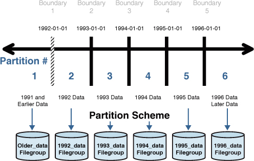
Notice that SalesBigPF1 is referenced as the partition function in Listing 2. This ties together the partition scheme and partition function. Figure 1
shows how the partitions defined in the function would be mapped to the
filegroup(s). At this point, you have made no changes to any table, and
you have not even specified the column in the table that you will
partition. The next section discusses those details.