1. Characterizing I/O workload
To determine an
application's ideal storage system and disk quantity, it's important to
understand the type and volume of I/O the application will generate.
This section focuses on the different types of I/O, the metrics used to
classify workload, and methods used in measuring and estimating values
for the I/O metrics.
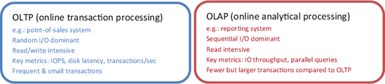
1.1. OLTP vs. OLAP/DSS
When classifying the nature of I/O, two main terms are used: OLTP and OLAP. An example of an OLTP
database is one that stores data for a point-of-sales application,
typically consisting of a high percentage of simple, short transactions
from a large number of users. Such transactions generate what's referred
to as random I/O, where the physical disks spend a significant percentage of time seeking data from various parts of the disk for read and/or write purposes.
In contrast, as shown in figure 1, an OLAP, or decision support system
(DSS), database is one that stores data for reporting applications that
usually have a smaller number of users generating much larger queries.
Such queries typically result in sequential
I/O, where the physical disks spend most of their time scanning a range
of data clustered together in the same part of the disk. Unlike OLTP
databases, OLAP databases typically have a much higher percentage of
read activity.
Note that even for classic
OLTP applications such as point-of-sales systems, actions like backups
and database consistency checks will still generate large amounts of
sequential I/O. For the purposes of I/O workload classification, we'll
consider the main I/O pattern only.
As you'll see a little
later, the difference between sequential and random I/O has an important
bearing on the storage system design.
1.2. I/O metrics
To design a storage system for a database application, in addition to knowing the type of workload it produces (OLTP or OLAP), we need to know the volume of workload, typically measured by the number of disk reads and writes per second.
The process of
obtaining or deriving these figures is determined by the state of the
application. If the application is an existing production system, the
figures can be easily obtained using Windows Performance Monitor.
Alternatively, if the system is yet to be commissioned, estimates are
derived using various methods. A common one is to use a test environment
to profile the reads and writes per transaction type, and then multiply
by the expected number of transactions per second per type.
Existing systems
We'll focus on the methods used to collect and analyze system
bottlenecks, including disk I/O bottlenecks. For the purposes of this
section, let's assume that disk I/O is determined to be a significant
bottleneck and we need to redesign the storage system to correct it. The
task, then, is to collect I/O metrics to assist in this process.
We can use the Windows Performance Monitor tool to collect the disk I/O metrics we need. For each logical disk
volume—that is, the drive letter corresponding to a data or log
drive—the following counters, among others, can be collected:
Note that the averages of these values should be collected during the database's peak usage
period. Designing a system based on weekly averages that include long
periods of very low usage may result in the system being overwhelmed
during the most important period of the day.
In the next section, we'll use these values to approximate the number of physical disks required for optimal I/O performance.
New systems
For a system not yet in
production, application I/O is estimated per transaction type in an
isolated test environment. Projections are then made based on the
estimated maximum number of expected transactions per second, with an
adjustment made for future growth.
Armed with these
metrics, let's proceed to the next section, where we'll use them to
project the estimated number of disks required to design a
high-performance storage system capable of handling the application
load.
2. Determining the required number of disks and controllers
In the previous section, we
covered the process of measuring, or estimating, the number of database
disk reads and writes generated by an application per second. In this
section, we'll cover the formula used to estimate the number of disks
required to design a storage system capable of handling the expected
application I/O load.
Note that
the calculations presented in this section are geared toward
direct-attached storage (DAS) solutions using traditional RAID storage.
Configuring SAN-based Virtualized RAID (V-RAID) storage is a specialist
skill, and one that differs among various SAN solutions and vendors.
Therefore, use the calculations presented here as a rough guideline
only.
2.1. Calculating the number of disks required
In calculating the
number of disks required to support a given workload, we must know two
values: the required disk I/O per second (which is the sum of the reads
and writes that we looked at in the previous section) and the I/O per
second capacity (IOPS) of the individual disks involved.
The IOPS value of a given
disk depends on many factors, such as the type of disk, spin speed, seek
time, and I/O type. While tools such as SQLIO, can be used to measure a disk's IOPS capacity, an often-used
average is 125 IOPS per disk for random I/O. Despite the fact that
commonly used server class 15,000 RPM SCSI disks are capable of higher
speeds,
the 125 IOPS figure is a reasonable average for the purposes of
estimation and enables the calculated disk number to include a
comfortable margin for handling peak, or higher than expected, load.
|
The process of
selecting RAID levels and calculating the required number of disks is
significantly different in a SAN compared to a traditional
direct-attached storage (DAS) solution. Configuring and monitoring
virtualized SAN storage is a specialist skill. Unless already skilled in
building SAN solutions, DBAs should insist on SAN vendor involvement in
the setup and configuration of storage for SQL Server deployments. The
big four SAN vendors (EMC, Hitachi, HP, and IBM) are all capable of
providing their own consultants, usually well versed in SQL Server
storage requirements, to set up and configure storage and related backup
solutions to maximize SAN investment.
|
Here's a commonly used formula for calculating required disk numbers:
Required # Disks = (Reads/sec + (Writes/sec * RAID adjuster)) / Disk IOPS
Dividing the sum of the
disk reads and writes per second by the disk's IOPS yields the number of
disks required to support the workload. As an example, let's assume we
need to design a RAID 10 storage system to support 1,200 reads per
second and 400 writes per second. Using our formula, the number of
required disks (assuming 125 IOPS per disk) can be calculated as
follows:
Required # disks = (1200 + (400 * 2)) / 125 = 16 DISKS
Note the doubling of
the writes per second figure (400 * 2); in this example, we're designing
a RAID 10 volume, and as you'll see in a moment, two physical writes
are required for each logical write—hence the adjustment to the writes
per second figure. Also note that this assumes the disk volume will be
dedicated to the application's database. Combining multiple databases on
the one disk will obviously affect the calculations.
Although this is a
simple example, it highlights the important relationship between the
required throughput, the IOPS capacity of the disks, and the number of
disks required to support the workload.
Finally, a crucial aspect of disk configuration, is the separation of the transaction log and data files. Unlike random
access within data files, transaction logs are written in a sequential
manner, so storing them on the same disk as data files will result in
reduced transaction throughput, with the disk heads moving between the
conflicting requirements of random and sequential I/O. In contrast,
storing the transaction log on a dedicated disk will enable the disk
heads to stay in position, writing sequentially, and therefore increase
the transaction throughput.
Once we've determined the number of disks required, we need to ensure the I/O bus has adequate bandwidth.
|
Here are some typical storage formats used by SQL Server systems:
ATA—Using
a parallel interface, ATA is one of the original implementations of
disk drive technologies for the personal computer. Also known as IDE or
parallel ATA, it integrates the disk controller on the disk itself and
uses ribbon-style cables for connection to the host.
SATA—In
widespread use today, SATA, or serial ATA, drives are an evolution of
the older parallel ATA drives. They offer numerous improvements such as
faster data transfer, thinner cables for better air flow, and a feature
known as Native Command Queuing (NCQ) whereby queued disk requests are
reordered to maximize the throughput. Compared to SCSI drives, SATA
drives offer much higher capacity per disk, with terabyte drives (or
higher) available today. The downside of very large SATA disk sizes is
the increased latency of disk requests, partially offset with NCQ.
SCSI—Generally
offering higher performance than SATA drives, albeit for a higher cost,
SCSI drives are commonly found in server-based RAID implementations and
high-end workstations. Paired with a SCSI controller card, up to 15
disks (depending on the SCSI version) can be connected to a server for
each channel on the controller card. Dual-channel cards enable 30 disks
to be connected per card, and multiple controller cards can be installed
in a server, allowing a large number of disks to be directly attached
to a server. It's increasingly common for organizations to use a mixture
of both SCSI drives for performance-sensitive applications and SATA
drives for applications requiring high amounts of storage. An example of
this for a database application is to use SCSI drives for storing the
database and SATA drives for storing online disk backups.
SAS—Serial
Attached SCSI (SAS) disks connect directly to a SAS port, unlike
traditional SCSI disks, which share a common bus. Borrowing from aspects
of Fibre Channel technology, SAS was designed to break past the current
performance barrier of the existing Ultra320 SCSI technology, and
offers numerous advantages owing to its smaller form factor and backward
compatibility with SATA disks. As a result, SAS drives are growing in
popularity as an alternative to SCSI.
Fibre Channel—Fibre
Channel allows high-speed, serial duplex communications between storage
systems and server hosts. Typically found on SANs, Fibre Channel offers
more flexibility than a SCSI bus, with support for more physical disks,
more connected servers, and longer cable lengths.
Solid-state disks—Used
today primarily in laptops and consumer devices, solid-state disks
(SSDs) are gaining momentum in the desktop and server space. As the name
suggests, SSDs use solid-state memory to persist data in contrast to
rotating platters in a conventional hard disk. With no moving parts,
SSDs are more robust and promise near-zero seek time, high performance,
and low power consumption.
|
2.2. Bus bandwidth
When designing a
storage system with many physical disks to support a large number of
reads and writes, we must consider the ability of the I/O bus to handle
the throughput.
As you learned in the previous section, typical OLTP applications consist of random I/O with a moderate percentage of disk time seeking data, with disk latency
(the time between disk request and response) an important factor. In
contrast, OLAP applications spend a much higher percentage of time
performing sequential I/O—thus the throughput is greater and bandwidth
requirements are higher.
In a direct-attached SCSI disk enclosure, the typical bus used today is Ultra320,
with a maximum throughput of 320MB/second per channel. Alternatively, a
2 Gigabit Fibre Channel system offers approximately 400MB/second
throughput in full duplex mode.
In our example of 2,000
disk transfers per second, assuming these were for an OLTP application
with random I/O and 8K I/O transfers (the SQL Server transfer size for
random I/O), the bandwidth requirements can be calculated as 2,000 times
8K, which is a total of 16MB/second, well within the capabilities of
either Ultra320 SCSI or 2 Gigabit Fibre Channel.
Should the
bandwidth requirements exceed the maximum throughput, additional disk
controllers and/or channels will be required to support the load. OLAP
applications typically have much higher throughput requirements, and
therefore have a lower disk to bus ratio, which means more
controllers/channels for the same number of disks.
You'll note that
we haven't addressed storage capacity requirements yet. This is a
deliberate decision to ensure the storage system is designed for
throughput and performance as the highest priority.
2.3. A note on capacity
A common mistake
made when designing storage for SQL Server databases is to base the
design on capacity requirements alone. A guiding principle in designing
high-performance storage solutions for SQL Server is to stripe data
across a large number of dedicated disks and multiple controllers. The
resultant performance is much greater than what you'd achieve with
fewer, higher-capacity disks. Storage solutions designed in this manner
usually exceed the capacity requirements as a consequence of the
performance-centric approach.
In our previous example
(where we calculated the need for 16 disks), assuming we use 73GB disks,
we have a total available capacity of 1.1TB. Usable space, after RAID
10 is implemented, would come down to around 500GB.
If the projected capacity requirements for our database only total 50GB, then so be it.
We end up with 10 percent storage utilization as a consequence of a
performance-centric design. In contrast, a design that was capacity-centric
would probably choose a single 73GB disk, or two disks to provide
redundancy. What are the consequences of this for our example? Assuming
125 IOPS per disk, we'd experience extreme disk bottlenecks with massive
disk queues handling close to 2,000 required IOPS!
While low
utilization levels will probably be frowned upon, this is the price of
performance, and a much better outcome than constantly dealing with disk
bottlenecks. A quick look at any of the server specifications used in
setting performance records for the Transaction Processing Performance
Council (tpc.org) tests will confirm a low-utilization, high-disk-stripe
approach like the one I described.
Finally,
placing capacity as a secondary priority behind performance doesn't mean
we can ignore it. Sufficient work should be carried out to estimate
both the initial and future storage requirements. Running out of disk
space at 3 a.m. isn't something I recommend!
In this section, I've
made a number of references to various RAID levels used to provide disk
fault tolerance. In the next section, we'll take a closer look at the
various RAID options and their pros and cons for use in a SQL Server
environment.