Excel names the functions that pertain to the normal
distribution so that you can tell whether you’re dealing with any normal
distribution, or the unit normal distribution with a mean of 0 and a
standard deviation of 1.
Excel refers to the unit normal distribution as the “standard” normal, and therefore uses the letter s
in the function’s name. So the NORM.DIST() function refers to any
normal distribution, whereas the NORMSDIST() compatibility function and
the NORM.S.DIST() consistency function refer specifically to the unit
normal distribution.
The NORM.DIST() Function
Suppose you’re
interested in the distribution in the population of high-density
lipoprotein (HDL) levels in adults over 20 years of age. That variable
is normally measured in milligrams per deciliter of blood (mg/dl).
Assuming HDL levels are normally distributed (and they are), you can
learn more about the distribution of HDL in the population by applying
your knowledge of the normal curve. One way to do so is by using Excel’s
NORM.DIST() function.
NORM.DIST() Syntax
The NORM.DIST() function takes the following data as its arguments:
x—
This is a value in the distribution you’re evaluating. If you’re
evaluating high-density lipoprotein (HDL) levels, you might be
interested in one specific level—say, 60. That specific value is the one
you would provide as the first argument to NORM.DIST().
Mean—
The second argument is the mean of the distribution you’re evaluating.
Suppose that the mean HDL among humans over 20 years of age is 54.3.
Standard Deviation—
The third argument is the standard deviation of the distribution you’re
evaluating. Suppose that the standard deviation of HDL levels is 15.
Cumulative— The
fourth argument indicates whether you want the cumulative probability
of HDL levels from 0 to x (which we’re taking to be 56 in this example),
or the probability of having an HDL level of specifically x (that is,
56). If you want the cumulative probability, use TRUE as the fourth
argument. If you want the specific probability, use FALSE.
Requesting the Cumulative Probability
The formula
=NORM.DIST(60, 54.3, 15, TRUE)
returns .648, or 64.8%. This means that 64.8% of the area under the distribution of HDL levels is between 0 and 60 mg/dl. Figure 1 shows this result.
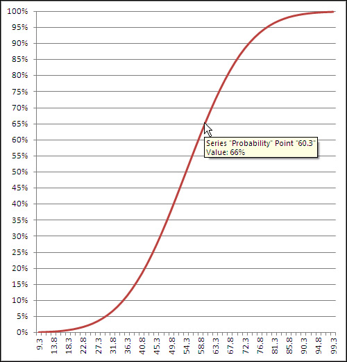
If you hover your mouse
pointer over the line that shows the cumulative probability, you’ll see a
small pop-up window that tells you which data point you are pointing
at, as well as its location on both the horizontal and vertical axes.
Once created, the chart can tell you the probability associated with any
of the charted data points, not just the 60 mg/dl this section has
discussed. As shown in Figure 1,
you can use either the chart’s gridlines or your mouse pointer to
determine that a measurement of, for example, 60.3 mg/dl or below
accounts for about 66% of the population.
Requesting the Point Estimate
Things
are different if you choose FALSE as the fourth, cumulative argument to
NORM.DIST(). In that case, the function returns the probability
associated with the specific point you specify in the first argument.
Use the value FALSE for the cumulative argument if you want to know the
height of the normal curve at a specific value of the distribution
you’re evaluating. Figure 2 shows one way to use NORM.DIST() with the cumulative argument set to FALSE.
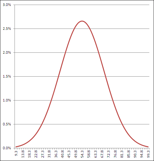
It doesn’t often happen that
you need a point estimate of the probability of a specific value in a
normal curve, but if you do—for example, to draw a curve that helps you
or someone else visualize an outcome—then setting the cumulative
argument to FALSE is a good way to get it. (You might also see this
value—the probability of a specific point, the height of the curve at
that point—referred to as the probability density function or probability mass function. The terminology has not been standardized.)
If you’re using a version of Excel
prior to 2010, you can use the NORMDIST() compatibility function. It is
the same as NORM.DIST() as to both arguments and returned values.
The NORM.INV() Function
As a practical matter, you’ll find
that you usually have need for the NORM.DIST() function after the fact.
That is, you have collected data and know the mean and standard
deviation of a sample or population. A question then arises: Where does a
given value fall in a normal distribution? That value might be a sample
mean that you want to compare to a population, or it might be an
individual observation that you want to assess in the context of a
larger group.
In that case, you would pass
the information along to NORM.DIST(), which would tell you the
probability of observing up to a particular value (cumulative = TRUE) or
that specific value (cumulative = FALSE). You could then compare that
probability to the alpha rate that you already adopted for your
experiment.
The NORM.INV() function
is closely related to the NORM.DIST() function and gives you a slightly
different angle on things. Instead of returning a value that represents
an area—that is, a probability—NORM.INV() returns a value that
represents a point on the normal curve’s horizontal axis. That’s the
point that you provide as the first argument to NORM.DIST().
For example, the prior section showed that the formula
=NORM.DIST(60, 54.3, 15, TRUE)
returns .648. The value 60 is
at least as large as 64.8% of the observations in a normal distribution
that has a mean of 54.3 and a standard deviation of 15.
The other side of the coin: the formula
=NORM.INV(0.648, 54.3, 15)
returns 60. If your distribution
has a mean of 54.3 and a standard deviation of 15, then 64.8% of the
distribution lies at or below a value of 60. That illustration is just,
well, illustrative. You would not normally care that 64.8% of a
distribution lies below a particular value.
But suppose that in
preparation for a research project you decide that you will conclude
that a treatment has a reliable effect only if the mean of the
experimental group is in the top 5% of the population. In that case, you would want to know what score would define that top 5%.
If you know the mean and
standard deviation, NORM.INV() does the job for you. Still taking the
population mean at 54.3 and the standard deviation at 15, the formula
=NORM.INV(0.95, 54.3, 15)
returns 78.97. Five percent of
a normal distribution that has a mean of 54.3 and a standard deviation
of 15 lies above a value of 78.97.
As
you see, the formula uses 0.95 as the first argument to NORM.INV().
That’s because NORM.INV assumes a cumulative probability—notice that
unlike NORM.DIST(), the NORM.INV() function has no fourth, cumulative
argument. So asking what value cuts off the top 5% of the distribution
is equivalent to asking what value cuts off the bottom 95% of the
distribution.
In this context, choosing to use
NORM.DIST() or NORM.INV() is largely a matter of the sort of
information you’re after. If you want to know how likely it is that you
will observe a number at least as large as X, hand X off to NORM.DIST()
to get a probability. If you want to know the number that serves as the
boundary of an area—an area that corresponds to a given probability—hand
the area off to NORM.INV() to get that number.
In either case, you need to
supply the mean and the standard deviation. In the case of NORM.DIST,
you also need to tell the function whether you’re interested in the
cumulative probability or the point estimate.
The consistency function
NORM.INV() is not available in versions of Excel prior to 2010, but you
can use the compatibility function NORMINV() instead. The arguments and
the results are as with NORM.INV().
Using NORM.S.DIST()
There’s much to be said
for expressing distances, weights, durations, and so on in their
original unit of measure. That’s what NORM.DIST() is for. But when you
want to use a standard unit of measure for a variable that’s distributed
normally, you should think of NORM.S.DIST(). The S in the middle of the function name of course stands for standard.
It’s quicker to use
NORM.S.DIST() because you don’t have to supply the mean or standard
deviation. Because you’re making reference to the unit normal
distribution, the mean (0) and the standard deviation (1) are known by
definition. All that NORM.S.DIST() needs is the z-score and whether you
want a cumulative area (TRUE) or a point estimate (FALSE). The function
uses this simple syntax:
=NORM.S.DIST(z, cumulative)
Thus, the formula
=NORM.S.DIST(1.5, TRUE)
informs you that 93.3% of the area under a normal curve is found to the left of a z-score of 1.5.
Caution
The
compatibility function NORMSDIST() is available in versions of Excel
prior to 2010. It is the only one of the normal distribution functions
whose argument list is different from that of its associated consistency
function. NORMSDIST() has no cumulative
argument: It returns by default the cumulative area to the left of the z
argument. Excel will warn that you have made an error if you supply a cumulative
argument to NORMSDIST(). If you want the point estimate rather than the
cumulative probability, you should use the NORMDIST() function with 0
as the second argument and 1 as the third. Those two together specify
the unit normal distribution, and you can now supply FALSE as the fourth
argument to NORMDIST(). Here’s an example:
=NORMDIST(1,0,1,FALSE)
Using NORM.S.INV()
It’s even simpler to use the inverse of NORM.S.DIST(), which is NORM.S.INV(). All the latter function needs is a probability:
=NORM.S.INV(.95)
This formula returns 1.64,
which means that 95% of the area under the normal curve lies to the left
of a z-score of 1.64. If you’ve taken a course in elementary
inferential statistics, that number probably looks familiar: as familiar
as the 1.96 that cuts off 97.5% of the distribution.
These are frequently
occurring numbers because they are associated with the
all-too-frequently occurring “p<.05” and “p<.025” entries at the
bottom of tables in journal reports—a rut that you don’t want to get
caught in.
The compatibility function NORMSINV() takes the same argument and returns the same result as does NORM.S.INV().
There is another Excel
worksheet function that pertains directly to the normal distribution:
CONFIDENCE.NORM(). To discuss the purpose and use of that function
sensibly, it’s necessary first to explore a little background.