A confidence interval
is a range of values that gives the user a sense of how precisely a
statistic estimates a parameter. The most familiar use of a confidence
interval is likely the “margin of error” reported in news stories about
polls: “The margin of error is plus or minus 3 percentage points.” But
confidence intervals are useful in contexts that go well beyond that
simple situation.
Confidence intervals can be
used with distributions that aren’t normal—that are highly skewed or in
some other way non-normal. But it’s easiest to understand what they’re
about in symmetric distributions, so the topic is introduced here. Don’t
let that get you thinking that you can use confidence intervals with
normal distributions only.
The Meaning of a Confidence Interval
Suppose that you measured the
HDL level in the blood of 100 adults on a special diet and calculated a
mean of 50 mg/dl with a standard deviation of 20. You’re aware that the
mean is a statistic, not a population parameter, and that another sample
of 100 adults, on the same diet, would very likely return a different
mean value. Over many repeated samples, the grand mean—that is, the mean
of the sample means—would turn out to be very, very close to the
population parameter.
But your resources don’t
extend that far and you’re going to have to make do with just the one
statistic, the 50 mg/dl that you calculated for your sample. Although
the value of 20 that you calculate for the sample standard deviation is a
statistic, it is the same as the known population standard deviation of
20. You can make use of the sample standard deviation and the number of
HDL values that you tabulated in order to get a sense of how much play
there is in that sample estimate.
You do so by constructing a
confidence interval around that mean of 50 mg/dl. Perhaps the interval
extends from 45 to 55. (And here you can see the relationship to “plus
or minus 3 percentage points.”) Does that tell you that the true
population mean is somewhere between 45 and 55?
No, it doesn’t, although it
might well be. Just as there are many possible samples that you might
have taken, but didn’t, there are many possible confidence intervals you
might have constructed around the sample means, but couldn’t. As you’ll
see, you construct your confidence interval in such a way that if you
took many more means and put confidence intervals around them, 95% of
the confidence intervals would capture the true population mean. As to
the specific confidence interval that you did construct, the probability
that the true population mean falls within the interval is either 1 or
0: either the interval captures the mean or it doesn’t.
However, it is more
rational to assume that the one confidence interval that you took is one
of the 95% that capture the population mean than to assume it doesn’t.
So you would tend to believe, with 95% confidence, that the interval is
one of those that captures the population mean.
Although I’ve spoken of
95% confidence intervals in this section, you can also construct 90% or
99% confidence intervals, or any other degree of confidence that makes
sense to you in a particular situation. You’ll see next how your choices
when you construct the interval affect the nature of the interval
itself. It turns out that it smoothes the discussion if you’re willing
to suspend your disbelief a bit, and briefly: I’m going to ask you to
imagine a situation in which you know what the standard deviation of a
measure is in the population, but that you don’t know its mean in the
population. Those circumstances are a little odd but far from
impossible.
Constructing a Confidence Interval
A confidence interval on a mean, as described in the prior section, requires these building blocks:
The mean itself
The standard deviation of the observations
The number of observations in the sample
The level of confidence you want to apply to the confidence interval
Starting with the level
of confidence, suppose that you want to create a 95% confidence
interval: You want to construct it in such a way that if you created 100
confidence intervals, 95 of them would capture the true population
mean.
In that case, because you’re dealing with a normal distribution, you could enter these formulas in a worksheet:
=NORM.S.INV(0.025)
=NORM.S.INV(0.975)
The NORM.S.INV() function,
described in the prior section, returns the z-score that has to its left
the proportion of the curve’s area given as the argument. Therefore,
NORM.S.INV(0.025) returns −1.96. That’s the z-score that has 0.025, or
2.5%, of the curve’s area to its left.
Similarly, NORM.S.INV(0.975)
returns 1.96, which has 97.5% of the curve’s area to its left. Another
way of saying it is that 2.5% of the curve’s area lies to its right.
These figures are shown in Figure 1.
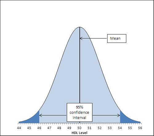
The area under the curve in Figure 1,
and between the values 46.1 and 53.9 on the horizontal axis, accounts
for 95% of the area under the curve. The curve, in theory, extends to
infinity to the left and to the right, so all possible values for the
population mean are included in the curve. Ninety-five percent of the
possible values lie within the 95% confidence interval between 46.1 and
53.9.
The figures 46.1 and 53.9
were chosen so as to capture that 95%. If you wanted a 99% confidence
interval (or some other interval more or less likely to be one of the
intervals that captures the population mean), you would choose different
figures. Figure 2 shows a 99% confidence interval around a sample mean of 50.
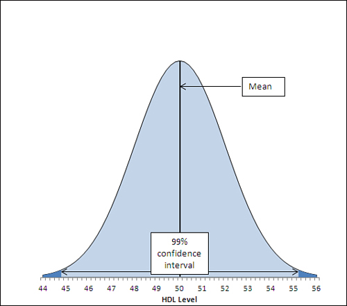
In Figure 2,
the 99% confidence interval extends from 44.8 to 55.2, a total of 2.6
points wider than the 95% confidence interval depicted in Figure 7.6.
If a hundred 99% confidence intervals were constructed around the means
of 100 samples, 99 of them (not 95 as before) would capture the
population mean. The additional confidence is provided by making the
interval wider. And that’s always the tradeoff in confidence intervals.
The narrower the interval, the more precisely you draw the boundaries,
but the fewer such intervals will capture the statistic in question
(here, that’s the mean). The broader the interval, the less precisely
you set the boundaries but the larger the number of intervals that
capture the statistic.
Other than setting the
confidence level, the only factor that’s under your control is the
sample size. You generally can’t dictate that the standard deviation is
to be smaller, but you can take larger samples. The standard deviation used in a confidence interval around a sample
mean is not the standard deviation of the individual raw scores. It is
that standard deviation divided by the square root of the sample size,
and this is known as the standard error of the mean.
The data set used to create the charts in Figures 1 and 2
has a standard deviation of 20, known to be the same as the population
standard deviation. The sample size is 100. Therefore, the standard
error of the mean is
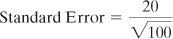
or 2.
To complete the
construction of the confidence interval, you multiply the standard error
of the mean by the z-scores that cut off the confidence level you’re
interested in. Figure 7.6,
for example, shows a 95% confidence interval. The interval must be
constructed so that 95% lies under the curve and within the
interval—therefore, 5% must lie outside the interval, with 2.5% divided
equally between the tails.
Here’s where the NORM.S.INV() function comes into play. Earlier in this section, these two formulas were used:
=NORM.S.INV(0.025)
=NORM.S.INV(0.975)
They return the z-scores
−1.96 and 1.96, which form the boundaries for 2.5% and 97.5% of the unit
normal distribution, respectively. If you multiply each by the standard
error of 2, and add the sample mean of 50, you get 46.1 and 53.9, the
limits of a 95% confidence interval on a mean of 50 and a standard error
of 2.
If you want a 99% confidence interval, use the formulas
=NORM.S.INV(0.005)
=NORM.S.INV(0.995)
to return −2.58 and 2.58. These
z-scores cut off one half of one percent of the unit normal distribution
at each end. The remainder of the area under the curve is 99%.
Multiplying each z-score by 2 and adding 50 for the mean results in 44.8
and 55.2, the limits of a 99% confidence interval on a mean of 50 and a
standard error of 2.
At this point it can help to
back away from the arithmetic and focus instead on the concepts. Any
z-score is some number of standard deviations—so a z-score of 1.96 is a
point that’s found at 1.96 standard deviations above the mean, and a
z-score of −1.96 is found 1.96 standard deviations below the mean.
Because the nature of the normal
curve has been studied so extensively, we know that 95% of the area
under a normal curve is found between 1.96 standard deviations below the
mean and 1.96 standard deviations above the mean.
When you want to put a confidence
interval around a sample mean, you start by deciding what percentage of
other sample means, if collected and calculated, you would want to fall
within that interval. So, if you decided that you wanted 95% of
possible sample means to be captured by your confidence interval, you
would put it 1.96 standard deviations above and below your sample mean.
But how large is the relevant
standard deviation? In this situation, the relevant units are themselves
mean values. You need to know the standard deviation not of the
original and individual observations, but of the means that are
calculated from those observations. That standard deviation has a
special name, the standard error of the mean.
Because of mathematical derivations and
long experience with the way the numbers behave, we know that a good,
close estimate of the standard deviation of the mean values is the
standard deviation of individual scores, divided by the square root of
the sample size. That’s the standard deviation you want to use to
determine your confidence interval.
In the example this
section has explored, the standard deviation is 20 and the sample size
is 100, so the standard error of the mean is 2. When you calculate 1.96
standard errors below the mean of 50 and above the mean of 50, you wind
up with values of 46.1 and 53.9. That’s your 95% confidence interval. If
you took another 99 samples from the population, 95 of 100 similar
confidence intervals would capture the population mean. It’s sensible to
conclude that the confidence interval you calculated is one of the 95
that capture the population mean. It’s not sensible to conclude that
it’s one of the remaining 5 that don’t.