Microsoft Excel 2010 : Using Excel with the Normal Distribution - The Central Limit Theorem

Your data collectors return with a total of 517,000 two-minute vehicle counts. The counts are accurately tabulated (that’s more fairy tale, but that’s also the end of it) and entered into an Excel worksheet. You create an Excel pivot chart as shown in Figure 1 to get a preliminary sense of the scope of the observations.

Figure 1. To keep things manageable, the number of vehicles is grouped by tens.

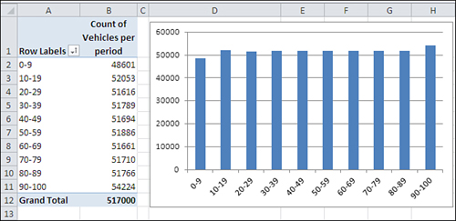
In Figure 1, different ranges of vehicles are shown as “row labels” in A2:A11. So, for example, there were 48,601 instances of between 0 and 9 vehicles crossing intersections within two-minute periods. Your data collectors recorded another 52,053 instances of between 10 and 19 vehicles crossing intersections within a two-minute period.

Notice that the data follows a uniform, rectangular distribution. Every grouping (for example, 0 to 9, 10 to 19, and so on) contains roughly the same number of observations.

Next, you calculate and chart the mean observation of each of the 2,500 intersections. The result appears in Figure 2.

Figure 2. Charting means converts a rectangular distribution to a normal distribution.

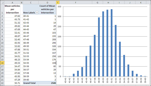
Perhaps you expected the outcome shown in Figure 7.13, perhaps not. Most people don’t. The underlying distribution is rectangular. There are as many intersections in your city that are traversed by zero to ten vehicles per two-minute period as there are intersections that attract 90 to 100 vehicles per two-minute period.

But if you take samples from that set of 510,000 observations, calculate the mean of each sample, and plot the results, you get something close to a normal distribution.

And this is termed the Central Limit Theorem. Take samples from a population that is distributed in any way: rectangular, skewed, binomial, bimodal, whatever (it’s rectangular in Figure 7.12). Get the mean of each sample and chart a frequency distribution of the means (refer to Figure 7.13). The chart of the means will resemble a normal distribution.

The larger the sample size, the closer the approximation to the normal distribution. The means in Figure 7.13 are based on samples of 100 each. If the samples had contained, say, 200 observations each, the chart would have come even closer to a normal distribution.

Making Things Easier

During the first half of the twentieth century, great reliance was placed on the Central Limit Theorem as a way to calculate probabilities. Suppose you want to investigate the prevalence of left-handedness among golfers. You believe that 10% of the general population is left-handed. You have taken a sample of 1,500 golfers and want to reassure yourself that there isn’t some sort of systematic bias in your sample. You count the lefties and find 135. Assuming that 10% of the population is left-handed and that you have a representative sample, what is the probability of selecting 135 or fewer left-handed golfers in a sample of 1,500?

The formula that calculates that exact probability is

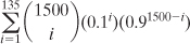
or, as you might write the formula using Excel functions:

=SUM(COMBIN(1500,ROW(A1:A135))*(0.1^ROW(A1:A135))* (0.9^(1500-ROW(A1:A135))))

(The formula must be array-entered in Excel, using Ctrl+Shift+Enter instead of simply Enter.)

That’s formidable, whether you use summation notation or Excel function notation. It would take a long time to calculate its result by hand, in part because you’d have to calculate 1,500 factorial.

When mainframe and mini computers became broadly accessible in the 1970s and 1980s, it became feasible to calculate the exact probability, but unless you had a job as a programmer, you still didn’t have the capability on your desktop.

When Excel came along, you could make use of BINOMDIST(), and in Excel 2010 BINOM.DIST(). Here’s an example:

=BINOM.DIST(135,1500,0.1,TRUE)

Any of those formulas returns the exact binomial probability, 10.48%. (That figure may or may not make you decide that your sample is nonrepresentative; it’s a subjective decision.) But even in 1950 there wasn’t much computing power available. You had to rely, so I’m told, on slide rules and compilations of mathematical and scientific tables to get the job done and come up with something close to the 10.48% figure.

Alternatively, you could call on the Central Limit Theorem. The first thing to notice is that a dichotomous variable such as handedness—right-handed versus left-handed—has a standard deviation just as any numeric variable has a standard deviation. If you let p stand for one proportion such as 0.1 and (1 − p) stand for the other proportion, 0.9, then the standard deviation of that variable is as follows:

That is, the square root of the product of the two proportions, such that they sum to 1.0. With a sample of some number n of people who possess or lack that characteristic, the standard deviation of that number of people is

and the standard deviation of a distribution of the handedness of 1,500 golfers, assuming 10% lefties and 90% righties, would be

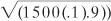
or 11.6.

You know what the number of golfers in your sample who are left-handed should be: 10% of 1,500, or 150. You know the standard deviation, 11.6. And the Central Limit Theorem tells you that the means of many samples follow a normal distribution, given that the samples are large enough. Surely 1,500 is a large sample.

Therefore, you should be able to compare your finding of 135 left-handed golfers with the normal distribution. The observed count of 135, less the mean of 150, divided by the standard deviation of 11.6, results in a z-score of −1.29. Any table that shows areas under the normal curve—and that’s any elementary statistics textbook—will tell you that a z-score of −1.29 corresponds to an area, a probability, of 9.84%. In the absence of a statistics textbook, you could use either

=NORM.S.DIST(−1.29,TRUE)

or, equivalently

=NORM.DIST(135,150,11.6,TRUE)

The result of using the normal distribution is 9.84%. The result of using the exact binomial distribution is 10.48: slightly over half a percent difference.

Making Things Better

The 9.84% figure is called the “normal approximation to the binomial.” It was and to some degree remains a popular alternative to using the binomial itself. It used to be popular because calculating the nCr combinations formula was so laborious and error prone. The approximation is still in some use because not everyone who has needed to calculate a binomial probability since the mid-1980s has had access to the appropriate software. And then there’s cognitive inertia to contend with.

That slight discrepancy between 9.84% and 10.48% is the sort that statisticians have in past years referred to as “negligible,” and perhaps it is. However, other constraints have been placed on the normal approximation method, such as the advice not to use it if either np or n(1−p) is less than 5. Or, depending on the source you read, less than 10. And there has been contentious discussion in the literature about the use of a “correction for continuity,” which is meant to deal with the fact that things such as counts of golfers go up by 1 (you can’t have 3/4 of a golfer) whereas things such as kilograms and yards are infinitely divisible. So the normal approximation to the binomial, prior to the accessibility of the huge amounts of computing power we now enjoy, was a mixed blessing.

The normal approximation to the binomial hangs its hat on the Central Limit Theorem. Largely because it has become relatively easy to calculate the exact binomial probability, you see normal approximations to the binomial less and less. The same is true of other approximations. The Central Limit Theorem remains a cornerstone of statistical theory, but (as far back as 1970) a nationally renowned statistician wrote that it “does not play the crucial role it once did.”